Terrain Shadows: The Bilbao Valley
This page is the rendered output of a Jupyter notebook that ships in the repository, together with all the data it uses. To run it yourself, see Running the tutorials.
Most thermal comfort studies take place on flat or gently sloping urban terrain. Bilbao is different: the city sits in a narrow river valley (the Nervión), flanked by hills that rise 200–400 m above the valley floor within just a few kilometres.
This creates a shadow geometry that standard flat-city models miss entirely — hillsides block the early-morning sun from the valley floor in summer, while east- and west-facing slopes receive sharply asymmetric radiation all day.
This tutorial demonstrates:
- Loading a normalised DSM (building heights above ground) with a separate DEM using
dsm_relative=True - Why
max_shadow_distance_mmatters in hilly terrain — and how to choose it - How terrain shadows create asymmetric sun exposure across a valley
- Visualising a terrain profile to understand the geometry
Data sources:
- BDSM/CDSM/DEM: Derived from PNOA-LiDAR point cloud data. Instituto Geográfico Nacional (IGN), Spain. Licence: CC BY 4.0.
- EPW weather: EnergyPlus Weather Data, U.S. Department of Energy.
from pathlib import Path

import matplotlib.pyplot as plt
import numpy as np
import solweig

# Resolve the repo root so this notebook runs from the repo root or docs/tutorials/
ROOT = next(p for p in [Path.cwd(), *Path.cwd().parents] if (p / "demos").exists())

DATA_DIR = ROOT / "demos/data/bilbao"
WORK_DIR = Path("temp/tutorial_cache/bilbao")
WORK_DIR.mkdir(parents=True, exist_ok=True)

assert (DATA_DIR / "BDSM.tif").exists(), f"Demo data not found at {DATA_DIR.resolve()}"

# 3 km × 3 km extract: Casco Viejo, Nervión riverfront, and flanking hillsides
# EPSG:25830 (ETRS89 / UTM zone 30N)
EXTENTS_BBOX = [499600, 4794000, 502600, 4797000]
1. Inspect the terrain
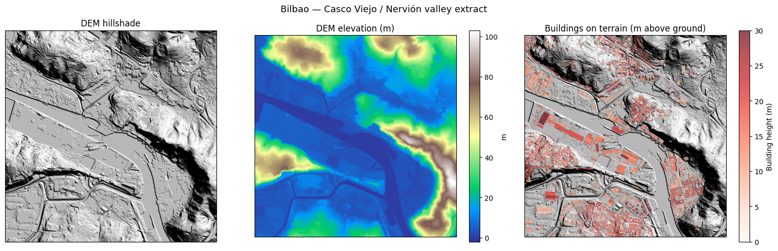
Before running any calculation, let's understand the landscape. The DEM contains terrain elevation; the BDSM contains building heights above ground (normalised DSM). Together they describe the full height geometry of the scene.
dem, dem_transform, dem_crs, _ = solweig.io.load_raster(str(DATA_DIR / "DEM.tif"))
bdsm, bdsm_transform, _, _ = solweig.io.load_raster(str(DATA_DIR / "BDSM.tif"))

print(f"DEM  shape: {dem.shape}  range: {np.nanmin(dem):.0f} – {np.nanmax(dem):.0f} m")
print(f"BDSM shape: {bdsm.shape}  building heights: 0 – {np.nanmax(bdsm):.0f} m above ground")

# Simple hillshade from DEM gradients
sun_az, sun_el = np.radians(225), np.radians(45)
dy, dx = np.gradient(dem)
slope = np.arctan(np.sqrt(dx**2 + dy**2))
aspect = np.arctan2(-dy, dx)
hillshade = np.clip(
    np.sin(sun_el) * np.cos(slope) + np.cos(sun_el) * np.sin(slope) * np.cos(sun_az - aspect),
    0,
    1,
)

fig, axes = plt.subplots(1, 3, figsize=(16, 5))

im0 = axes[0].imshow(hillshade, cmap="gray")
axes[0].set_title("DEM hillshade")

im1 = axes[1].imshow(dem, cmap="terrain")
axes[1].set_title("DEM elevation (m)")
plt.colorbar(im1, ax=axes[1], label="m")

# Resample BDSM to DEM grid for overlay (nearest-neighbour)
bdsm_ds = bdsm[::2, ::2]  # BDSM is 2× the DEM resolution
h, w = dem.shape
bdsm_ds = bdsm_ds[:h, :w]
building_mask = np.where(bdsm_ds > 0.5, bdsm_ds, np.nan)
axes[2].imshow(hillshade, cmap="gray")
im2 = axes[2].imshow(building_mask, cmap="Reds", alpha=0.7, vmin=0, vmax=30)
axes[2].set_title("Buildings on terrain (m above ground)")
plt.colorbar(im2, ax=axes[2], label="Building height (m)")

for ax in axes:
    ax.set_xticks([])
    ax.set_yticks([])
plt.suptitle("Bilbao — Casco Viejo / Nervión valley extract", fontsize=13)
plt.tight_layout()
plt.show()
DEM  shape: (680, 680)  range: -2 – 103 m
BDSM shape: (1359, 1359)  building heights: 0 – 52 m above ground
2. Valley cross-section
A north–south profile through the centre of the domain reveals the classic bowl shape: the Nervión river at the bottom, hillsides rising steeply on both sides.
mid_col = dem.shape[1] // 2
profile = dem[:, mid_col]
pixel_size_dem = 5.0  # DEM at ~5 m resolution
distance_m = np.arange(len(profile)) * pixel_size_dem

fig, ax = plt.subplots(figsize=(12, 4))
ax.fill_between(distance_m, profile, alpha=0.4, color="saddlebrown", label="Terrain")
ax.plot(distance_m, profile, color="saddlebrown", linewidth=1.5)
ax.set_xlabel("Distance south → north (m)")
ax.set_ylabel("Elevation (m)")
ax.set_title("N–S terrain cross-section through the Nervión valley (centre of domain)")
ax.annotate(
    "Nervión river\n(valley floor)",
    xy=(distance_m[np.argmin(profile)], profile.min()),
    xytext=(distance_m[np.argmin(profile)] - 400, profile.min() + 20),
    arrowprops=dict(arrowstyle="->"),
    fontsize=9,
)
plt.tight_layout()
plt.show()

print(f"Relief across domain: {profile.max() - profile.min():.0f} m over {distance_m[-1] / 1000:.1f} km")
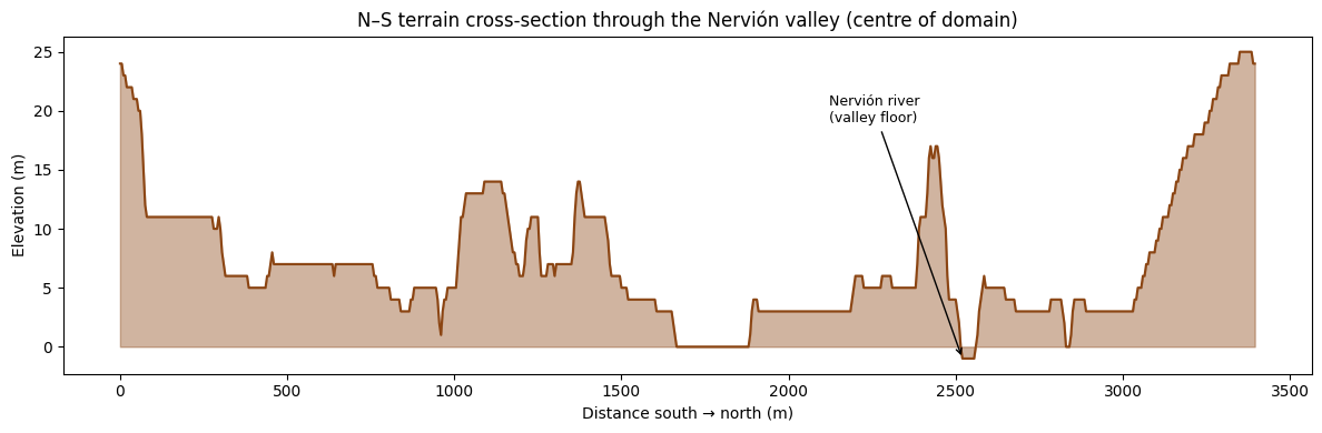
Relief across domain: 26 m over 3.4 km
3. Generate a land cover map
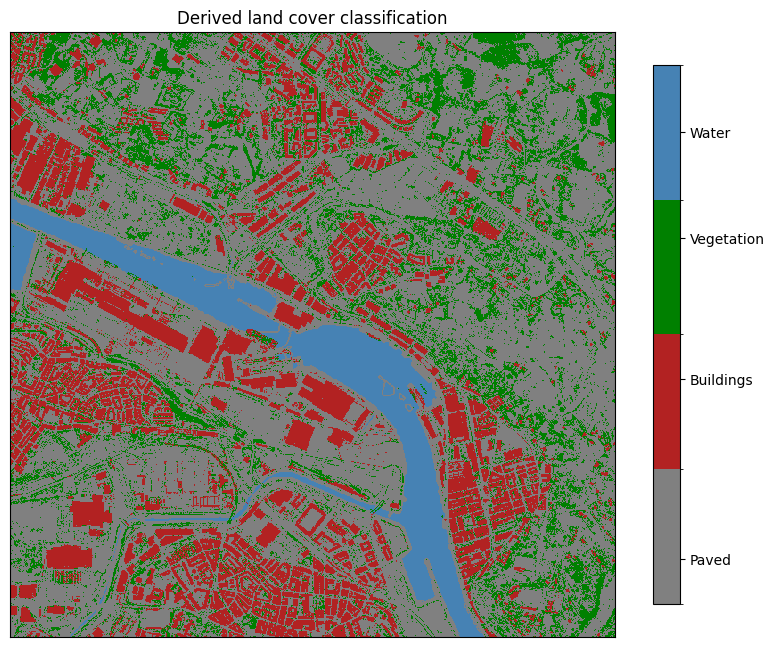
SOLWEIG uses land cover classes to assign surface properties (albedo, emissivity, thermal behaviour) that vary between asphalt, grass, water, etc. Without a land cover map everything defaults to paved/cobblestone — the Nervión river would have the same thermal properties as a car park.
We can derive a reasonable classification from the layers we already have:
| Source | Class | UMEP ID |
|---|---|---|
| BDSM > 0.5 m | Buildings | 2 |
| CDSM > 0.5 m (non-building) | Vegetation / grass | 5 |
| DEM: low-elevation flat areas in the valley floor | Water (Nervión) | 7 |
| Everything else | Paved / urban surface | 0 |
# Load CDSM (vegetation canopy heights)
cdsm, cdsm_transform, _, _ = solweig.io.load_raster(str(DATA_DIR / "CDSM.tif"))

# Start with paved (ID 0) everywhere
lc = np.zeros(dem.shape, dtype=np.uint8)

# Buildings (ID 2): where BDSM has height > 0.5 m
# Resample to DEM grid (BDSM is 2× DEM resolution)
bdsm_ds = bdsm[::2, ::2][: dem.shape[0], : dem.shape[1]]
lc[bdsm_ds > 0.5] = 2

# Vegetation (ID 5): where CDSM has canopy > 0.5 m and no building
cdsm_ds = cdsm[::2, ::2][: dem.shape[0], : dem.shape[1]]
veg_mask = (cdsm_ds > 0.5) & (lc != 2)
lc[veg_mask] = 5

# Water (ID 7): Nervión river — low elevation, flat terrain in the valley floor
dy, dx = np.gradient(dem)
slope_deg = np.degrees(np.arctan(np.sqrt(dx**2 + dy**2)))
water_mask = (dem < 1) & (slope_deg < 2) & (lc == 0)  # low, flat, not already classified
lc[water_mask] = 7

# Save as GeoTIFF (same grid as DEM)
lc_path = str(WORK_DIR / "land_cover.tif")
solweig.io.save_raster(lc_path, lc.astype(np.float32), dem_transform, dem_crs, no_data_val=255, generate_preview=False)

# Summary
unique, counts = np.unique(lc, return_counts=True)
lc_names = {0: "Paved", 2: "Buildings", 5: "Vegetation", 7: "Water"}
print("Land cover classification:")
for val, cnt in zip(unique, counts, strict=True):
    pct = 100 * cnt / lc.size
    print(f"  {lc_names.get(val, f'ID {val}'):12s} (ID {val}): {cnt:>8,} px  ({pct:.1f}%)")

# Visualise
lc_cmap = plt.matplotlib.colors.ListedColormap(["gray", "firebrick", "green", "steelblue"])
bounds = [-0.5, 1, 2.5, 6, 8]
norm = plt.matplotlib.colors.BoundaryNorm(bounds, lc_cmap.N)

fig, ax = plt.subplots(figsize=(8, 8))
im = ax.imshow(lc, cmap=lc_cmap, norm=norm, interpolation="nearest")
cbar = plt.colorbar(im, ax=ax, ticks=[0, 2, 5, 7], shrink=0.7)
cbar.ax.set_yticklabels(["Paved", "Buildings", "Vegetation", "Water"])
ax.set_title("Derived land cover classification")
ax.set_xticks([])
ax.set_yticks([])
plt.tight_layout()
plt.show()
Land cover classification:
  Paved        (ID 0):  268,142 px  (58.0%)
  Buildings    (ID 2):   86,847 px  (18.8%)
  Vegetation   (ID 5):   75,672 px  (16.4%)
  Water        (ID 7):   31,739 px  (6.9%)
4. Prepare the surface
The key difference from the Athens workflow: the BDSM contains relative building
heights (metres above ground, not above sea level). Setting dsm_relative=True tells
prepare() to compute the absolute DSM as DEM + BDSM before processing.
The land cover map generated above is passed in so that water and vegetation receive appropriate surface properties instead of defaulting to paved/cobblestone everywhere.
surface = solweig.SurfaceData.prepare(
    dsm=str(DATA_DIR / "BDSM.tif"),
    dem=str(DATA_DIR / "DEM.tif"),
    cdsm=str(DATA_DIR / "CDSM.tif"),
    land_cover=lc_path,
    working_dir=str(WORK_DIR / "working"),
    bbox=EXTENTS_BBOX,
    pixel_size=2.5,
    dsm_relative=True,  # BDSM is height above ground — DEM provides the baseline
)

print(f"Surface shape: {surface.dsm.shape}")
print(f"Pixel size:    {surface.pixel_size} m")
print(f"Absolute DSM:  {np.nanmin(surface.dsm):.0f} – {np.nanmax(surface.dsm):.0f} m (terrain + buildings)")
print(f"Land cover:    {'yes' if surface.land_cover is not None else 'no'}")
solweig.models.surface: Fast-path cache invalidated (1 change):


solweig.models.surface:   - source 'land_cover' mtime changed (1783364243 → 1783368440)


solweig.models.surface: Rebuilding from source rasters…


solweig.models.surface: Preparing surface data from GeoTIFF files...


solweig.models.surface_loading:   DSM: 1359×1359 pixels


solweig.models.surface_loading:   Using specified pixel size: 2.50 m


solweig.models.surface_loading:   CRS validated: ETRS89 / UTM zone 30N (EPSG:25830)


solweig.models.surface_loading:   ✓ Canopy DSM (CDSM) provided


solweig.models.surface_loading:   ✓ Ground elevation (DEM) provided


solweig.models.surface_loading:   → No TDSM provided - will auto-generate from CDSM (ratio=0.25)


solweig.io: No-data value is 255.0, replacing with NaN


solweig.models.surface_loading:   ✓ Land cover provided (albedo/emissivity derived from classification)


solweig.models.surface_loading: Checking for preprocessing data...


solweig.io: No-data value is -9999.0, replacing with NaN


solweig.io: No-data value is -9999.0, replacing with NaN


solweig.models.surface_loading:   ✓ Walls found in working_dir: temp/tutorial_cache/bilbao/working/walls/px2.500


solweig.models.surface_loading:   ✓ SVF loaded from memmap (memory-efficient)


solweig.models.surface_loading:   ✓ SVF found in working_dir: temp/tutorial_cache/bilbao/working/svf/px2.500


solweig.models.surface_loading:   ✓ Shadow matrices loaded from npz


solweig.models.surface_loading:   ✓ Shadow matrices found (anisotropic sky enabled)


solweig.models.surface_loading: Computing spatial extent and resolution...


solweig.models.surface_loading:   Using user-specified extent: [499600, 4794000, 502600, 4797000]


solweig.models.surface_loading:   ✓ Resampled to 1200×1200 pixels


solweig.models.surface_loading:   Layers loaded: DSM, CDSM, DEM, land_cover


solweig.models.surface: Smoothing quantized DEM (Q=1.00m, sigma=3.0px) to suppress stair-step SVF artifacts over gently sloped terrain


solweig.models.surface: Converting relative DSM to absolute: DSM = DEM + nDSM


solweig.models.surface: Flattened 33339 DSM pixels below 1.0m nDSM to DEM (removing sub-threshold features)


solweig.models.surface: Auto-generating TDSM from CDSM using trunk_ratio=0.25


solweig.models.surface: Converted relative CDSM to absolute (base: DEM)


solweig.models.surface: Converted relative TDSM to absolute (base: DEM)


solweig.models.surface: Cleared 9397 vegetation pixels below DSM (canopy was underground)


solweig.models.surface:   Valid mask: all pixels valid


solweig.models.surface:   Crop: no trimming needed (valid bbox = full extent)


solweig.models.surface:   Cleaned rasters saved to temp/tutorial_cache/bilbao/working/cleaned


solweig.models.surface: ✓ Surface data prepared successfully


Surface shape: (1200, 1200)
Pixel size:    2.5 m
Absolute DSM:  -1 – 101 m (terrain + buildings)
Land cover:    yes
5. Load weather
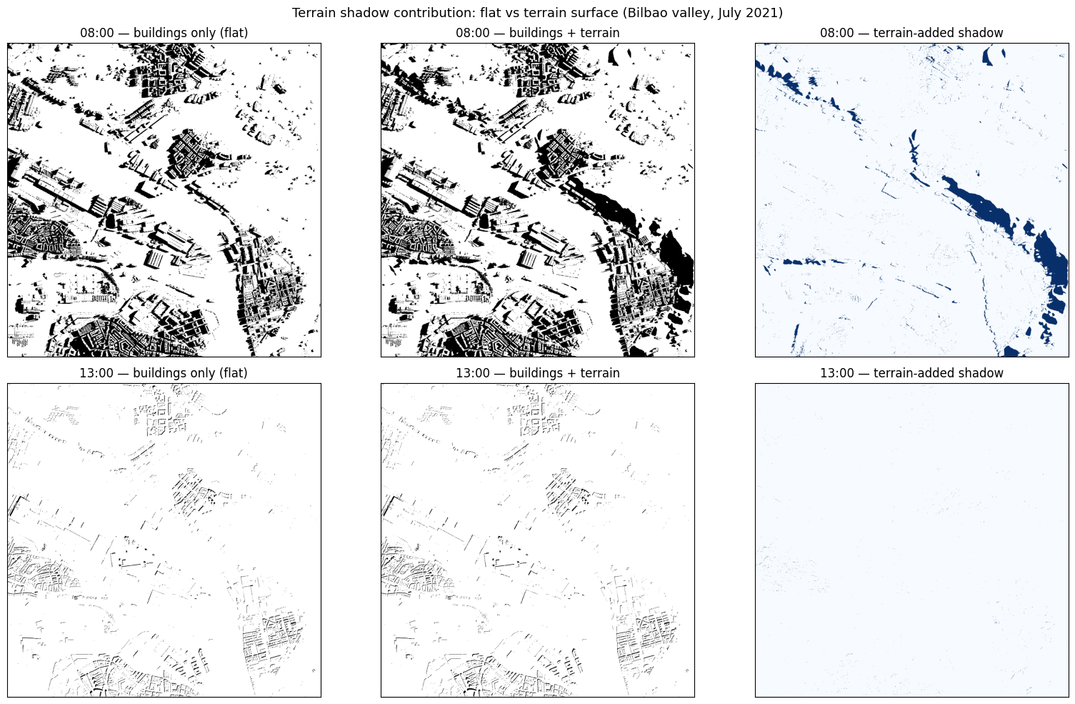
We use a single clear summer morning (08:00 on July 2nd) — when the sun is still low in the east and terrain shadows across the valley are at their most dramatic.
epw_path = str(DATA_DIR / "bilbao_2021.epw")
weather_list = solweig.Weather.from_epw(epw_path, start="2021-07-02", end="2021-07-02")
location = solweig.Location.from_epw(epw_path)

lon_hemisphere = "E" if location.longitude >= 0 else "W"
print(f"Location: {location.latitude:.2f}°N, {abs(location.longitude):.2f}°{lon_hemisphere}")

# Pick 08:00 (low morning sun) and 13:00 (high sun near solar noon)
w_08h = next(w for w in weather_list if w.datetime.hour == 8)
w_13h = next(w for w in weather_list if w.datetime.hour == 13)

for w in [w_08h, w_13h]:
    print(f"  {w.datetime:%H:%M}  Ta={w.ta:.1f}°C  RH={w.rh:.0f}%  GlobRad={w.global_rad:.0f} W/m²")
solweig.io_epw: Loaded EPW file: unknown, 8760 timesteps (pure Python parser)


solweig.models.weather: Loaded 24 timesteps from EPW: 2021-07-02 00:00 → 2021-07-02 23:00


solweig.models.location: Location from EPW: unknown — 43.2926°N, -2.9728°E (UTC+1, -3m)


Location: 43.29°N, 2.97°W
  08:00  Ta=17.1°C  RH=87%  GlobRad=367 W/m²
  13:00  Ta=23.0°C  RH=69%  GlobRad=918 W/m²
6. Terrain shadow contribution: flat vs terrain surface
To isolate terrain shadows properly, we run the same timestep twice:
- Flat surface — BDSM treated as absolute building heights on flat ground (no DEM). Only buildings cast shadow.
- Terrain surface — full surface with DEM + BDSM. Buildings and hillsides cast shadow.
The difference between the two shadow maps is the pure terrain contribution — unconfounded by building shadow length or sun angle.
import tempfile

# Flat baseline: buildings on flat ground, no terrain
surface_flat = solweig.SurfaceData.prepare(
    dsm=str(DATA_DIR / "BDSM.tif"),
    working_dir=str(WORK_DIR / "working_flat"),
    bbox=EXTENTS_BBOX,
    pixel_size=2.5,
    # No DEM, no dsm_relative — BDSM values treated as absolute heights on flat ground
)

# Terrain surface: DEM + relative building heights — hills and buildings cast shadow
surface_terrain = solweig.SurfaceData.prepare(
    dsm=str(DATA_DIR / "BDSM.tif"),
    working_dir=str(WORK_DIR / "working_terrain"),
    bbox=EXTENTS_BBOX,
    pixel_size=2.5,
    dem=str(DATA_DIR / "DEM.tif"),
    dsm_relative=True,
)


def compute_shadow(sfc, weather_step, label):
    """Run a single-timestep shadow calculation and return the shadow grid."""
    with tempfile.TemporaryDirectory(prefix="solweig-bilbao-") as tmpdir:
        solweig.calculate(
            surface=sfc,
            weather=[weather_step],
            location=location,
            output_dir=tmpdir,
            outputs=["shadow"],
            max_shadow_distance_m=1000,
        )
        shadow_files = list(Path(tmpdir).glob("shadow/*.tif"))
        shadow, *_ = solweig.io.load_raster(str(shadow_files[0]))
    print(f"  {label}: shaded fraction = {(shadow < 0.5).mean():.1%}")
    return shadow


print("08:00 (low morning sun):")
shadow_08_flat = compute_shadow(surface_flat, w_08h, "flat (buildings only)")
shadow_08_terrain = compute_shadow(surface_terrain, w_08h, "terrain + buildings")

print("\n13:00 (near solar noon):")
shadow_13_flat = compute_shadow(surface_flat, w_13h, "flat (buildings only)")
shadow_13_terrain = compute_shadow(surface_terrain, w_13h, "terrain + buildings")
solweig.models.surface: Fast-path cache hit — loading prepared surface from temp/tutorial_cache/bilbao/working_flat


solweig.models.surface: Loading prepared surface from temp/tutorial_cache/bilbao/working_flat/cleaned


solweig.io: No-data value is -9999.0, replacing with NaN


solweig.models.surface:   DSM: 1200×1200 pixels


solweig.io: No-data value is -9999.0, replacing with NaN


solweig.io: No-data value is -9999.0, replacing with NaN


solweig.models.precomputed:   Loaded SVF memmap cache from temp/tutorial_cache/bilbao/working_flat/svf/px2.500/memmap


solweig.models.precomputed:   Loaded shadow matrices from temp/tutorial_cache/bilbao/working_flat/svf/px2.500/shadowmats.npz


solweig.models.precomputed:   Loaded SVF data: (1200, 1200)


solweig.models.precomputed:   Loaded shadow matrices for anisotropic sky


solweig.models.surface:   Loaded: DSM, walls, SVF, shadows


solweig.models.surface: Fast-path cache hit — loading prepared surface from temp/tutorial_cache/bilbao/working_terrain


solweig.models.surface: Loading prepared surface from temp/tutorial_cache/bilbao/working_terrain/cleaned


solweig.io: No-data value is -9999.0, replacing with NaN


solweig.models.surface:   DSM: 1200×1200 pixels


solweig.io: No-data value is -9999.0, replacing with NaN


solweig.io: No-data value is -9999.0, replacing with NaN


solweig.io: No-data value is -9999.0, replacing with NaN


solweig.models.precomputed:   Loaded SVF memmap cache from temp/tutorial_cache/bilbao/working_terrain/svf/px2.500/memmap


solweig.models.precomputed:   Loaded shadow matrices from temp/tutorial_cache/bilbao/working_terrain/svf/px2.500/shadowmats.npz


solweig.models.precomputed:   Loaded SVF data: (1200, 1200)


solweig.models.precomputed:   Loaded shadow matrices for anisotropic sky


solweig.models.surface:   Loaded: DSM, DEM, walls, SVF, shadows


08:00 (low morning sun):


solweig.tiling: Resource-aware tile sizing (context=solweig): GPU budget=30,150,672,384 bytes, RAM=11,007,016,960 available of 51,539,607,552 total, max_tile_side=3709 px


solweig.timeseries: ============================================================


solweig.timeseries: Starting SOLWEIG timeseries calculation


solweig.timeseries:   Grid size: 1200x1200 pixels


solweig.timeseries:   Timesteps: 1


solweig.timeseries:   Period: 2021-07-02 08:00 -> 2021-07-02 08:00


solweig.timeseries:   Location: 43.29N, -2.97E


solweig.timeseries: ============================================================


solweig.timeseries: Pre-computing sun positions and radiation splits...


solweig.timeseries:   Pre-computed 1 timesteps in 0.0s


[GPU] Shadow GPU context initialized successfully
SOLWEIG timeseries: 0%| | 0/1 [00:00<?, ?it/s]
[GPU] GVF GPU context initialized


[GPU] Anisotropic sky GPU context initialized
SOLWEIG timeseries: 100%|██████████| 1/1 [00:00<00:00, 1.47it/s]
SOLWEIG timeseries: 100%|██████████| 1/1 [00:00<00:00, 1.40it/s]
solweig.timeseries: ============================================================


solweig.timeseries: Calculation complete: 1 timesteps processed


solweig.timeseries:   Total time: 0.7s (1.35 steps/s)


solweig.timeseries: ============================================================


  flat (buildings only): shaded fraction = 20.4%
solweig.timeseries: ============================================================


solweig.timeseries: Starting SOLWEIG timeseries calculation


solweig.timeseries:   Grid size: 1200x1200 pixels


solweig.timeseries:   Timesteps: 1


solweig.timeseries:   Period: 2021-07-02 08:00 -> 2021-07-02 08:00


solweig.timeseries:   Location: 43.29N, -2.97E


solweig.timeseries: ============================================================


solweig.timeseries: Pre-computing sun positions and radiation splits...


solweig.timeseries:   Pre-computed 1 timesteps in 0.0s
SOLWEIG timeseries: 0%| | 0/1 [00:00<?, ?it/s]
SOLWEIG timeseries: 100%|██████████| 1/1 [00:00<00:00, 2.19it/s]
SOLWEIG timeseries: 100%|██████████| 1/1 [00:00<00:00, 2.10it/s]
solweig.timeseries: ============================================================


solweig.timeseries: Calculation complete: 1 timesteps processed


solweig.timeseries:   Total time: 0.5s (2.00 steps/s)


solweig.timeseries: ============================================================


  terrain + buildings: shaded fraction = 24.7%

13:00 (near solar noon):
solweig.timeseries: ============================================================


solweig.timeseries: Starting SOLWEIG timeseries calculation


solweig.timeseries:   Grid size: 1200x1200 pixels


solweig.timeseries:   Timesteps: 1


solweig.timeseries:   Period: 2021-07-02 13:00 -> 2021-07-02 13:00


solweig.timeseries:   Location: 43.29N, -2.97E


solweig.timeseries: ============================================================


solweig.timeseries: Pre-computing sun positions and radiation splits...


solweig.timeseries:   Pre-computed 1 timesteps in 0.0s
SOLWEIG timeseries: 0%| | 0/1 [00:00<?, ?it/s]
SOLWEIG timeseries: 100%|██████████| 1/1 [00:00<00:00, 2.50it/s]
SOLWEIG timeseries: 100%|██████████| 1/1 [00:00<00:00, 2.38it/s]
solweig.timeseries: ============================================================


solweig.timeseries: Calculation complete: 1 timesteps processed


solweig.timeseries:   Total time: 0.4s (2.23 steps/s)


solweig.timeseries: ============================================================


  flat (buildings only): shaded fraction = 2.3%
solweig.timeseries: ============================================================


solweig.timeseries: Starting SOLWEIG timeseries calculation


solweig.timeseries:   Grid size: 1200x1200 pixels


solweig.timeseries:   Timesteps: 1


solweig.timeseries:   Period: 2021-07-02 13:00 -> 2021-07-02 13:00


solweig.timeseries:   Location: 43.29N, -2.97E


solweig.timeseries: ============================================================


solweig.timeseries: Pre-computing sun positions and radiation splits...


solweig.timeseries:   Pre-computed 1 timesteps in 0.0s
SOLWEIG timeseries: 0%| | 0/1 [00:00<?, ?it/s]
SOLWEIG timeseries: 100%|██████████| 1/1 [00:00<00:00, 2.65it/s]
SOLWEIG timeseries: 100%|██████████| 1/1 [00:00<00:00, 2.49it/s]
solweig.timeseries: ============================================================


solweig.timeseries: Calculation complete: 1 timesteps processed


solweig.timeseries:   Total time: 0.4s (2.38 steps/s)


solweig.timeseries: ============================================================


  terrain + buildings: shaded fraction = 2.3%
fig, axes = plt.subplots(2, 3, figsize=(16, 10))

kw = dict(cmap="gray", vmin=0, vmax=1)

axes[0, 0].imshow(shadow_08_flat, **kw)
axes[0, 0].set_title("08:00 — buildings only (flat)")

axes[0, 1].imshow(shadow_08_terrain, **kw)
axes[0, 1].set_title("08:00 — buildings + terrain")

# Shadow grids are 1 = sunlit, 0 = shaded, so flat − terrain is 1 where
# the terrain adds shadow that the buildings alone would not cast.
terrain_shadow_08 = shadow_08_flat - shadow_08_terrain
axes[0, 2].imshow(terrain_shadow_08, cmap="Blues", vmin=0, vmax=1)
axes[0, 2].set_title("08:00 — terrain-added shadow")

axes[1, 0].imshow(shadow_13_flat, **kw)
axes[1, 0].set_title("13:00 — buildings only (flat)")

axes[1, 1].imshow(shadow_13_terrain, **kw)
axes[1, 1].set_title("13:00 — buildings + terrain")

terrain_shadow_13 = shadow_13_flat - shadow_13_terrain
axes[1, 2].imshow(terrain_shadow_13, cmap="Blues", vmin=0, vmax=1)
axes[1, 2].set_title("13:00 — terrain-added shadow")

for ax in axes.flat:
    ax.set_xticks([])
    ax.set_yticks([])

plt.suptitle(
    "Terrain shadow contribution: flat vs terrain surface (Bilbao valley, July 2021)",
    fontsize=13,
)
plt.tight_layout()
plt.show()
7. Multi-day summary: valley sun exposure
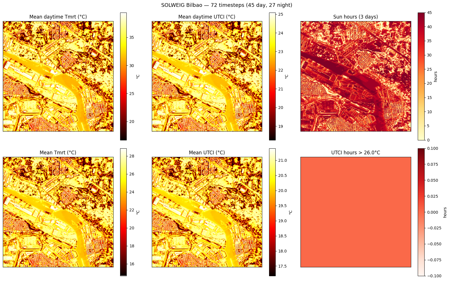
Running a 3-day timeseries (including nighttime hours) lets us build up the accumulated sun-hour map and compare daytime vs overall thermal conditions — the most revealing outputs for understanding how valley geometry drives long-term thermal comfort across the area.
all_weather = solweig.Weather.from_epw(epw_path, start="2021-07-01", end="2021-07-03")
print(f"Timesteps: {len(all_weather)} ({len(all_weather) // 3} per day × 3 days)")

OUTPUT_DIR = WORK_DIR / "output_valley"

summary = solweig.calculate(
    surface=surface,
    weather=all_weather,
    location=location,
    output_dir=str(OUTPUT_DIR),
    outputs=["tmrt", "shadow"],
    max_shadow_distance_m=500,
)
print(summary.report())
solweig.io_epw: Loaded EPW file: unknown, 8760 timesteps (pure Python parser)


solweig.models.weather: Loaded 72 timesteps from EPW: 2021-07-01 00:00 → 2021-07-03 23:00


Timesteps: 72 (24 per day × 3 days)
solweig.timeseries: ============================================================


solweig.timeseries: Starting SOLWEIG timeseries calculation


solweig.timeseries:   Grid size: 1200x1200 pixels


solweig.timeseries:   Timesteps: 72


solweig.timeseries:   Period: 2021-07-01 00:00 -> 2021-07-03 23:00


solweig.timeseries:   Location: 43.29N, -2.97E


solweig.timeseries: ============================================================


solweig.timeseries: Pre-computing sun positions and radiation splits...


solweig.timeseries:   Pre-computed 72 timesteps in 0.1s
SOLWEIG timeseries: 0%| | 0/72 [00:00<?, ?it/s]
SOLWEIG timeseries: 1%|▏ | 1/72 [00:00<00:46, 1.53it/s]
SOLWEIG timeseries: 3%|▎ | 2/72 [00:00<00:23, 3.03it/s]
SOLWEIG timeseries: 6%|▌ | 4/72 [00:00<00:12, 5.51it/s]
SOLWEIG timeseries: 8%|▊ | 6/72 [00:01<00:09, 7.26it/s]
SOLWEIG timeseries: 11%|█ | 8/72 [00:01<00:07, 8.10it/s]
SOLWEIG timeseries: 14%|█▍ | 10/72 [00:01<00:07, 8.79it/s]
SOLWEIG timeseries: 15%|█▌ | 11/72 [00:01<00:06, 9.01it/s]
SOLWEIG timeseries: 17%|█▋ | 12/72 [00:01<00:06, 9.14it/s]
SOLWEIG timeseries: 19%|█▉ | 14/72 [00:01<00:06, 9.53it/s]
SOLWEIG timeseries: 22%|██▏ | 16/72 [00:02<00:05, 9.73it/s]
SOLWEIG timeseries: 24%|██▎ | 17/72 [00:02<00:05, 9.69it/s]
SOLWEIG timeseries: 25%|██▌ | 18/72 [00:02<00:05, 9.45it/s]
SOLWEIG timeseries: 26%|██▋ | 19/72 [00:02<00:05, 9.11it/s]
SOLWEIG timeseries: 28%|██▊ | 20/72 [00:02<00:05, 9.16it/s]
SOLWEIG timeseries: 29%|██▉ | 21/72 [00:02<00:05, 9.25it/s]
SOLWEIG timeseries: 31%|███ | 22/72 [00:02<00:05, 9.33it/s]
SOLWEIG timeseries: 32%|███▏ | 23/72 [00:02<00:05, 9.47it/s]
SOLWEIG timeseries: 35%|███▍ | 25/72 [00:03<00:04, 9.83it/s]
SOLWEIG timeseries: 38%|███▊ | 27/72 [00:03<00:04, 10.16it/s]
SOLWEIG timeseries: 40%|████ | 29/72 [00:03<00:04, 10.11it/s]
SOLWEIG timeseries: 43%|████▎ | 31/72 [00:03<00:03, 10.55it/s]
SOLWEIG timeseries: 46%|████▌ | 33/72 [00:03<00:03, 10.11it/s]
SOLWEIG timeseries: 49%|████▊ | 35/72 [00:04<00:03, 10.13it/s]
SOLWEIG timeseries: 51%|█████▏ | 37/72 [00:04<00:03, 9.86it/s]
SOLWEIG timeseries: 54%|█████▍ | 39/72 [00:04<00:03, 9.88it/s]
SOLWEIG timeseries: 56%|█████▌ | 40/72 [00:04<00:03, 9.60it/s]
SOLWEIG timeseries: 57%|█████▋ | 41/72 [00:04<00:03, 9.66it/s]
SOLWEIG timeseries: 60%|█████▉ | 43/72 [00:04<00:03, 9.58it/s]
SOLWEIG timeseries: 61%|██████ | 44/72 [00:04<00:02, 9.63it/s]
SOLWEIG timeseries: 62%|██████▎ | 45/72 [00:05<00:02, 9.48it/s]
SOLWEIG timeseries: 64%|██████▍ | 46/72 [00:05<00:02, 9.56it/s]
SOLWEIG timeseries: 67%|██████▋ | 48/72 [00:05<00:02, 10.04it/s]
SOLWEIG timeseries: 69%|██████▉ | 50/72 [00:05<00:02, 10.18it/s]
SOLWEIG timeseries: 72%|███████▏ | 52/72 [00:05<00:01, 10.45it/s]
SOLWEIG timeseries: 75%|███████▌ | 54/72 [00:05<00:01, 10.41it/s]
SOLWEIG timeseries: 78%|███████▊ | 56/72 [00:06<00:01, 10.55it/s]
SOLWEIG timeseries: 81%|████████ | 58/72 [00:06<00:01, 10.28it/s]
SOLWEIG timeseries: 83%|████████▎ | 60/72 [00:06<00:01, 10.05it/s]
SOLWEIG timeseries: 86%|████████▌ | 62/72 [00:06<00:00, 10.19it/s]
SOLWEIG timeseries: 89%|████████▉ | 64/72 [00:06<00:00, 9.96it/s]
SOLWEIG timeseries: 90%|█████████ | 65/72 [00:07<00:00, 9.84it/s]
SOLWEIG timeseries: 92%|█████████▏| 66/72 [00:07<00:00, 9.83it/s]
SOLWEIG timeseries: 93%|█████████▎| 67/72 [00:07<00:00, 9.85it/s]
SOLWEIG timeseries: 94%|█████████▍| 68/72 [00:07<00:00, 9.84it/s]
SOLWEIG timeseries: 97%|█████████▋| 70/72 [00:07<00:00, 9.90it/s]
SOLWEIG timeseries: 99%|█████████▊| 71/72 [00:07<00:00, 9.88it/s]
SOLWEIG timeseries: 100%|██████████| 72/72 [00:07<00:00, 9.25it/s]
solweig.timeseries: ============================================================


solweig.timeseries: Calculation complete: 72 timesteps processed


solweig.timeseries:   Total time: 7.8s (9.22 steps/s)


solweig.timeseries: ============================================================


SOLWEIG Summary: 72 timesteps (45 day, 27 night)
  Period: 2021-07-01 00:00 — 2021-07-03 23:00
  Tmrt  — mean: 24.1°C, range: 6.6 – 66.2°C
  UTCI  — mean: 20.0°C, range: 13.3 – 34.6°C
  Sun   — 0.0 – 45.0 hours
  UTCI > 32°C (day) — max 6.0h
  Ta    — range: 13.3 – 23.0°C
  Summary GeoTIFFs: temp/tutorial_cache/bilbao/output_valley/summary/
    shade_hours.tif
    sun_hours.tif
    tmrt_day_mean.tif
    tmrt_max.tif
    tmrt_mean.tif
    tmrt_min.tif
    tmrt_night_mean.tif
    utci_day_mean.tif
    utci_hours_above_26_night.tif
    utci_hours_above_32_day.tif
    utci_hours_above_38_day.tif
    utci_max.tif
    utci_mean.tif
    utci_min.tif
    utci_night_mean.tif

Tip: per-timestep arrays are in summary.timeseries (e.g. .ta, .tmrt_mean, .utci_mean).
     Spatial grids are on the summary itself (e.g. .tmrt_mean, .utci_max).
     Summary grids are saved as GeoTIFFs above; timeseries arrays are in memory only.
fig, axes = plt.subplots(2, 3, figsize=(16, 10))

im0 = axes[0, 0].imshow(summary.tmrt_day_mean, cmap="hot")
axes[0, 0].set_title("Mean daytime Tmrt (°C)")
plt.colorbar(im0, ax=axes[0, 0], label="°C")

im1 = axes[0, 1].imshow(summary.utci_day_mean, cmap="hot")
axes[0, 1].set_title("Mean daytime UTCI (°C)")
plt.colorbar(im1, ax=axes[0, 1], label="°C")

im2 = axes[0, 2].imshow(summary.sun_hours, cmap="YlOrRd")
axes[0, 2].set_title("Sun hours (3 days)")
plt.colorbar(im2, ax=axes[0, 2], label="hours")

im3 = axes[1, 0].imshow(summary.tmrt_mean, cmap="hot")
axes[1, 0].set_title("Mean Tmrt (°C)")
plt.colorbar(im3, ax=axes[1, 0], label="°C")

im4 = axes[1, 1].imshow(summary.utci_mean, cmap="hot")
axes[1, 1].set_title("Mean UTCI (°C)")
plt.colorbar(im4, ax=axes[1, 1], label="°C")

threshold = sorted(summary.utci_hours_above.keys())[0]
im5 = axes[1, 2].imshow(summary.utci_hours_above[threshold], cmap="Reds")
axes[1, 2].set_title(f"UTCI hours > {threshold}°C")
plt.colorbar(im5, ax=axes[1, 2], label="hours")

for ax in axes.flat:
    ax.set_xticks([])
    ax.set_yticks([])

plt.suptitle(
    f"SOLWEIG Bilbao — {len(summary)} timesteps ({summary.n_daytime} day, {summary.n_nighttime} night)",
    fontsize=13,
)
plt.tight_layout()
plt.show()