Athens Quick Start: From GeoTIFFs to Tmrt Maps
This page is the rendered output of a Jupyter notebook that ships in the repository, together with all the data it uses. To run it yourself, see Running the tutorials.
This tutorial walks through a complete SOLWEIG workflow using real data from Athens, Greece. You'll load a Digital Surface Model, rasterise tree vectors, and compute a Mean Radiant Temperature (Tmrt) map for a hot July afternoon — all in a few lines of code.
Data sources:
- DSM/DEM: Derived from LiDAR data, Hellenic Cadastre (ktimatologio.gr)
- Tree vectors: Derived from Athens Urban Atlas (Copernicus) and geodata.gov.gr
- EPW weather: Generated via PVGIS using Copernicus Climate Change Service information [2025]. Neither the European Commission nor ECMWF is responsible for any use that may be made of the Copernicus information or data it contains.
from pathlib import Path

import geopandas as gpd
import matplotlib.pyplot as plt
import numpy as np
import solweig
from pyproj import CRS

# Resolve the repo root so this notebook runs from the repo root or docs/tutorials/
ROOT = next(p for p in [Path.cwd(), *Path.cwd().parents] if (p / "demos").exists())

# Paths — adjust if running from a different location
DATA_DIR = ROOT / "demos/data/athens"
WORK_DIR = ROOT / "temp/tutorial_cache"
WORK_DIR.mkdir(parents=True, exist_ok=True)

assert (DATA_DIR / "DSM.tif").exists(), f"Demo data not found at {DATA_DIR.resolve()}"

# Study area extents (EPSG:2100 — Greek Grid)
EXTENTS_BBOX = [476800, 4205850, 477200, 4206250]
TARGET_CRS = 2100
1. Inspect the Digital Surface Model
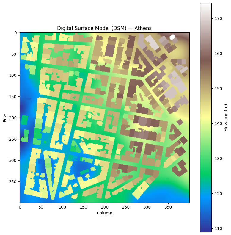
The DSM contains building and terrain heights. Let's load it and see what the study area looks like.
dsm, dsm_transform, dsm_crs, _ = solweig.io.load_raster(str(DATA_DIR / "DSM.tif"))

print(f"DSM shape: {dsm.shape}")
print(f"Height range: {np.nanmin(dsm):.1f} – {np.nanmax(dsm):.1f} m")
print(f"CRS: {dsm_crs}")

fig, ax = plt.subplots(figsize=(8, 8))
im = ax.imshow(dsm, cmap="terrain", vmin=np.nanmin(dsm), vmax=np.nanmax(dsm))
ax.set_title("Digital Surface Model (DSM) — Athens")
ax.set_xlabel("Column")
ax.set_ylabel("Row")
plt.colorbar(im, ax=ax, label="Elevation (m)")
plt.tight_layout()
plt.show()
solweig.io: No-data value is -9999.0, replacing with NaN


DSM shape: (400, 400)
Height range: 109.0 – 174.4 m
CRS: PROJCS["GGRS87 / Greek Grid",GEOGCS["GGRS87",DATUM["Greek_Geodetic_Reference_System_1987",SPHEROID["GRS 1980",6378137,298.257222101,AUTHORITY["EPSG","7019"]],AUTHORITY["EPSG","6121"]],PRIMEM["Greenwich",0,AUTHORITY["EPSG","8901"]],UNIT["degree",0.0174532925199433,AUTHORITY["EPSG","9122"]],AUTHORITY["EPSG","4121"]],PROJECTION["Transverse_Mercator"],PARAMETER["latitude_of_origin",0],PARAMETER["central_meridian",24],PARAMETER["scale_factor",0.9996],PARAMETER["false_easting",500000],PARAMETER["false_northing",0],UNIT["metre",1,AUTHORITY["EPSG","9001"]],AXIS["Easting",EAST],AXIS["Northing",NORTH],AUTHORITY["EPSG","2100"]]
2. Rasterise tree vectors into a Canopy DSM
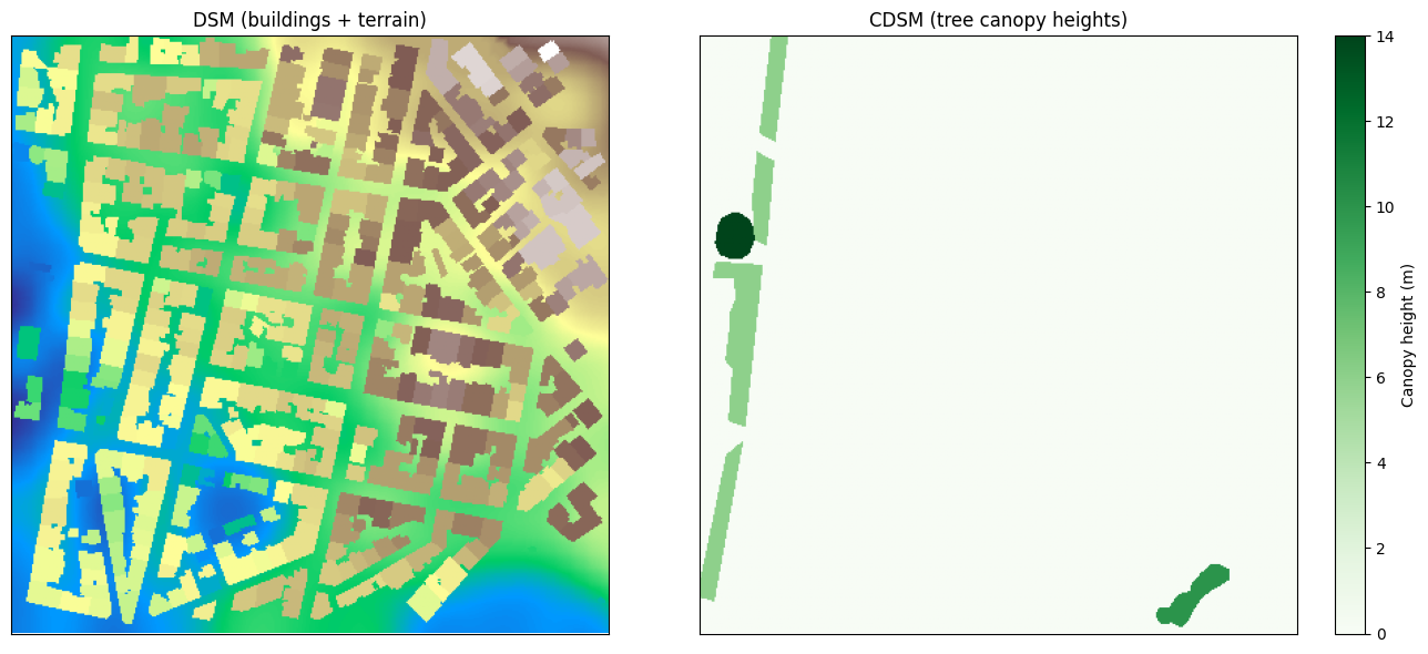
The Athens dataset includes a GeoPackage with tree polygon geometries and heights. We rasterise these to create a CDSM (Canopy Digital Surface Model) at 1 m resolution.
trees_gdf = gpd.read_file(str(DATA_DIR / "trees.gpkg"))
trees_gdf = trees_gdf.to_crs(TARGET_CRS)

print(f"Tree polygons: {len(trees_gdf)}")
print(f"Height range: {trees_gdf['height'].min():.1f} – {trees_gdf['height'].max():.1f} m")

cdsm_rast, cdsm_transf = solweig.io.rasterise_gdf(
    trees_gdf,
    "geometry",
    "height",
    bbox=EXTENTS_BBOX,
    pixel_size=1.0,
)

# Save so SurfaceData.prepare() can load it
cdsm_path = WORK_DIR / "CDSM.tif"
solweig.io.save_raster(
    str(cdsm_path),
    cdsm_rast,
    cdsm_transf.to_gdal(),
    CRS.from_epsg(TARGET_CRS).to_wkt(),
)

fig, axes = plt.subplots(1, 2, figsize=(14, 6))
axes[0].imshow(dsm, cmap="terrain")
axes[0].set_title("DSM (buildings + terrain)")
im1 = axes[1].imshow(cdsm_rast, cmap="Greens", vmin=0)
axes[1].set_title("CDSM (tree canopy heights)")
plt.colorbar(im1, ax=axes[1], label="Canopy height (m)")
for ax in axes:
    ax.set_xticks([])
    ax.set_yticks([])
plt.tight_layout()
plt.show()
Tree polygons: 6
Height range: 6.0 – 14.0 m
3. Prepare the surface
SurfaceData.prepare() loads the DSM and CDSM, computes wall heights and aspects,
calculates Sky View Factors (SVF), and caches everything in working_dir for reuse.
surface = solweig.SurfaceData.prepare(
    dsm=str(DATA_DIR / "DSM.tif"),
    working_dir=str(WORK_DIR / "working"),
    cdsm=str(cdsm_path),
    bbox=EXTENTS_BBOX,
    pixel_size=1.0,
)

print(f"Surface shape: {surface.dsm.shape}")
print(f"Pixel size: {surface.pixel_size} m")
solweig.models.surface: Fast-path cache invalidated (1 change):


solweig.models.surface:   - source 'cdsm' mtime changed (1783364226 → 1783368424)


solweig.models.surface: Rebuilding from source rasters…


solweig.models.surface: Preparing surface data from GeoTIFF files...


solweig.io: No-data value is -9999.0, replacing with NaN


solweig.models.surface_loading:   DSM: 400×400 pixels


solweig.models.surface_loading:   Using specified pixel size: 1.00 m


solweig.models.surface_loading:   CRS validated: GGRS87 / Greek Grid (EPSG:2100)


solweig.io: No-data value is -9999.0, replacing with NaN


solweig.models.surface_loading:   ✓ Canopy DSM (CDSM) provided


solweig.models.surface_loading:   → No TDSM provided - will auto-generate from CDSM (ratio=0.25)


solweig.models.surface_loading: Checking for preprocessing data...


solweig.io: No-data value is -9999.0, replacing with NaN


solweig.io: No-data value is -9999.0, replacing with NaN


solweig.models.surface_loading:   ✓ Walls found in working_dir: /Users/dev/repos/solweig/temp/tutorial_cache/working/walls/px1.000


solweig.models.surface_loading:   ✓ SVF loaded from memmap (memory-efficient)


solweig.models.surface_loading:   ✓ SVF found in working_dir: /Users/dev/repos/solweig/temp/tutorial_cache/working/svf/px1.000


solweig.models.surface_loading:   ✓ Shadow matrices loaded from npz


solweig.models.surface_loading:   ✓ Shadow matrices found (anisotropic sky enabled)


solweig.models.surface_loading: Computing spatial extent and resolution...


solweig.models.surface_loading:   Using user-specified extent: [476800, 4205850, 477200, 4206250]


solweig.models.surface_loading:   ✓ No resampling needed - all rasters match target grid


solweig.models.surface_loading:   Layers loaded: DSM, CDSM


solweig.models.surface: Auto-generating TDSM from CDSM using trunk_ratio=0.25


solweig.models.surface: Converted relative CDSM to absolute (base: DSM)


solweig.models.surface: Converted relative TDSM to absolute (base: DSM)


solweig.models.surface:   Valid mask: all pixels valid


solweig.models.surface:   Crop: no trimming needed (valid bbox = full extent)


solweig.models.surface:   Cleaned rasters saved to /Users/dev/repos/solweig/temp/tutorial_cache/working/cleaned


solweig.models.surface: ✓ Surface data prepared successfully


Surface shape: (400, 400)
Pixel size: 1.0 m
4. Load weather data
We load a single afternoon timestep from the Athens EPW file — July 1st at 14:00, a hot summer hour with strong solar radiation.
epw_path = str(DATA_DIR / "athens_2023.epw")
weather_list = solweig.Weather.from_epw(epw_path, start="2023-07-01", end="2023-07-01")
location = solweig.Location.from_epw(epw_path)

# Pick the 14:00 timestep
weather_14h = [w for w in weather_list if w.datetime.hour == 14][0]

print(f"Location: {location.latitude:.2f}°N, {location.longitude:.2f}°E")
print(f"Datetime: {weather_14h.datetime}")
print(f"Air temperature: {weather_14h.ta:.1f}°C")
print(f"Relative humidity: {weather_14h.rh:.0f}%")
print(f"Global radiation: {weather_14h.global_rad:.0f} W/m²")
print(f"Wind speed: {weather_14h.ws:.1f} m/s")
solweig.io_epw: Loaded EPW file: NA, 8760 timesteps (pure Python parser)


solweig.models.weather: Loaded 24 timesteps from EPW: 2023-07-01 00:00 → 2023-07-01 23:00


solweig.models.location: Location from EPW: NA — 38.0000°N, 23.7500°E (UTC+2, 175m)


Location: 38.00°N, 23.75°E
Datetime: 2023-07-01 14:00:00
Air temperature: 30.3°C
Relative humidity: 43%
Global radiation: 889 W/m²
Wind speed: 3.3 m/s
5. Calculate Tmrt
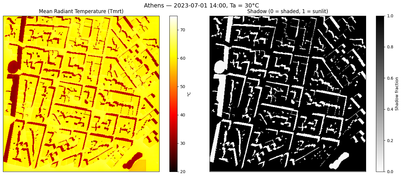
We run a single-timestep calculation using calculate() and save the outputs to disk.
OUTPUT_DIR = WORK_DIR / "output_quickstart"

summary = solweig.calculate(
    surface=surface,
    weather=[weather_14h],
    location=location,
    output_dir=str(OUTPUT_DIR),
    outputs=["tmrt", "shadow"],
)

# Load per-timestep outputs from disk
tmrt, *_ = solweig.io.load_raster(str(OUTPUT_DIR / "tmrt" / "tmrt_20230701_1400.tif"))
shadow, *_ = solweig.io.load_raster(str(OUTPUT_DIR / "shadow" / "shadow_20230701_1400.tif"))

fig, axes = plt.subplots(1, 2, figsize=(14, 6))

im0 = axes[0].imshow(tmrt, cmap="hot", vmin=20, vmax=75)
axes[0].set_title("Mean Radiant Temperature (Tmrt)")
plt.colorbar(im0, ax=axes[0], label="°C")

im1 = axes[1].imshow(shadow, cmap="gray_r", vmin=0, vmax=1)
axes[1].set_title("Shadow (0 = shaded, 1 = sunlit)")
plt.colorbar(im1, ax=axes[1], label="Shadow fraction")

for ax in axes:
    ax.set_xticks([])
    ax.set_yticks([])

plt.suptitle(f"Athens — {weather_14h.datetime:%Y-%m-%d %H:%M}, Ta = {weather_14h.ta:.0f}°C", fontsize=14)
plt.tight_layout()
plt.show()
solweig.tiling: Resource-aware tile sizing (context=solweig): GPU budget=30,150,672,384 bytes, RAM=11,279,073,280 available of 51,539,607,552 total, max_tile_side=3754 px


solweig.timeseries: ============================================================


solweig.timeseries: Starting SOLWEIG timeseries calculation


solweig.timeseries:   Grid size: 400x400 pixels


solweig.timeseries:   Timesteps: 1


solweig.timeseries:   Period: 2023-07-01 14:00 -> 2023-07-01 14:00


solweig.timeseries:   Location: 38.00N, 23.75E


solweig.timeseries: ============================================================


solweig.timeseries: Pre-computing sun positions and radiation splits...


solweig.timeseries:   Pre-computed 1 timesteps in 0.0s


[GPU] Shadow GPU context initialized successfully
SOLWEIG timeseries: 0%| | 0/1 [00:00<?, ?it/s]
[GPU] GVF GPU context initialized
[GPU] Anisotropic sky GPU context initialized
SOLWEIG timeseries: 100%|██████████| 1/1 [00:00<00:00, 10.54it/s]
solweig.timeseries: ============================================================


solweig.timeseries: Calculation complete: 1 timesteps processed


solweig.timeseries:   Total time: 0.1s (9.68 steps/s)


solweig.timeseries: ============================================================
6. Sun vs. shade
One of the most useful insights from SOLWEIG is the Tmrt difference between sunlit and shaded areas. This is the radiation benefit of shade — trees, buildings, or other structures.
sunlit_mask = shadow > 0.5
shaded_mask = shadow < 0.5

tmrt_sun = np.nanmean(tmrt[sunlit_mask])
tmrt_shade = np.nanmean(tmrt[shaded_mask])

print(f"Mean Tmrt (all):    {np.nanmean(tmrt):.1f}°C")
print(f"Mean Tmrt (sunlit): {tmrt_sun:.1f}°C")
print(f"Mean Tmrt (shaded): {tmrt_shade:.1f}°C")
print(f"Sun–shade difference: {tmrt_sun - tmrt_shade:.1f}°C")
Mean Tmrt (all):    56.2°C
Mean Tmrt (sunlit): 61.3°C
Mean Tmrt (shaded): 34.0°C
Sun–shade difference: 27.2°C