UDA-city Heat Risk Analysis

UDA-city is a synthetic hot-humid city with 10 neighbourhoods that differ in surface cover, building form, population exposure, and vulnerability. This analysis uses SUEWS to estimate neighbourhood heat hazard and then links that hazard to socio-economic heat risk. The main question is where heat-risk planning should be prioritised, not just which place is physically hottest.

Objective

To compare present and future neighbourhood heat risk in UDA-city, using SUEWS modelled heat hazard together with population exposure and vulnerability, and to identify where heat-risk planning should be prioritised.

Meteorological Forcing

The simulations use an hourly ERA5-derived hot-humid forcing for a synthetic coastal South Asian setting. The forcing period is 2024-03-02 01:00 to 2024-06-01 00:00 local time, with March used as model spin-up and April-May as the main hot-season analysis period.

The forcing variables used by SUEWS are air temperature (Tair), relative humidity (RH), wind speed (U), air pressure (pres), incoming shortwave radiation (kdown), incoming longwave radiation (ldown), and rainfall (rain). The present scenario uses the ERA5-derived forcing directly; the future scenario applies a uniform +2.5 C pseudo-warming to air temperature.

Neighbourhood Characteristics

UDA-city has 10 synthetic neighbourhoods. Surface fractions are from the canonical model input sidecar, and population density is in people per hectare. The deciduous-tree fraction is 0.000 for all neighbourhoods.

Grid	Neighbourhood	Type	Paved	Buildings	Evergreen trees	Grass	Bare soil	Water	Day pop.	Night pop.
1	Jade Gardens	refuge	0.593	0.047	0.108	0.072	0.100	0.080	80	100
2	Serendib Rise	refuge	0.572	0.068	0.108	0.072	0.100	0.080	80	100
3	Taman Melati	refuge	0.567	0.073	0.108	0.072	0.100	0.080	80	100
4	Kampong Lama	hotspot	0.710	0.140	0.030	0.020	0.080	0.020	300	400
5	Dhobi Lines	hotspot	0.680	0.170	0.030	0.020	0.080	0.020	300	400
6	Lusitano Square	core	0.600	0.200	0.060	0.040	0.050	0.050	250	130
7	Mlima Moto	hotspot	0.510	0.340	0.030	0.020	0.080	0.020	300	400
8	Victoria Exchange	core	0.460	0.340	0.060	0.040	0.050	0.050	250	130
9	Fuzhou Lanes	hotspot	0.500	0.350	0.030	0.020	0.080	0.020	300	400
10	Zheng He Towers	core	0.360	0.440	0.060	0.040	0.050	0.050	250	130

Methods

Heat hazard was calculated from SUEWS 2 m air temperature (T2) as the number of hours where hourly mean T2 > 35 C. These dangerous-heat hours were scaled from 0 to 1 across the 10 neighbourhoods. [risk_bridge.py, risk_bridge.md]
Exposure was calculated from daytime population density (population_day). Vulnerability was calculated from older people, young children, low AC access (1 - ac_access), outdoor workers, and deprivation. Both exposure and vulnerability were scaled from 0 to 1. [neighbourhoods.yml, socioeconomic.csv, risk_bridge.py]
Final heat risk was calculated by combining the scaled hazard, exposure, and vulnerability scores using a geometric mean: risk = (hazard x exposure x vulnerability)^(1/3). The final risk score was scaled from 0 to 1 and used to rank neighbourhoods. [risk_bridge.py, risk_bridge.md]

Heat Hazard and Risk Paradox for Present Scenario

Table 1. Present Scenario Heat Hazard and Risk Ranking

Grid	Neighbourhood	Type	Dangerous heat hours	Day pop.	Hazard	Exposure	Vulnerability	Risk index	Rank
4	Kampong Lama	hotspot	42	300	0.667	1.000	0.950	1.000	1
5	Dhobi Lines	hotspot	26	300	0.400	1.000	0.916	0.833	2
9	Fuzhou Lanes	hotspot	22	300	0.333	1.000	0.972	0.800	3
7	Mlima Moto	hotspot	5	300	0.050	1.000	1.000	0.429	4
6	Lusitano Square	core	5	250	0.050	0.773	0.089	0.176	5
8	Victoria Exchange	core	5	250	0.050	0.773	0.056	0.151	6
1	Jade Gardens	refuge	62	80	1.000	0.000	0.324	0.000	7
3	Taman Melati	refuge	47	80	0.750	0.000	0.363	0.000	7
2	Serendib Rise	refuge	26	80	0.400	0.000	0.274	0.000	7
10	Zheng He Towers	core	2	250	0.000	0.773	0.000	0.000	7

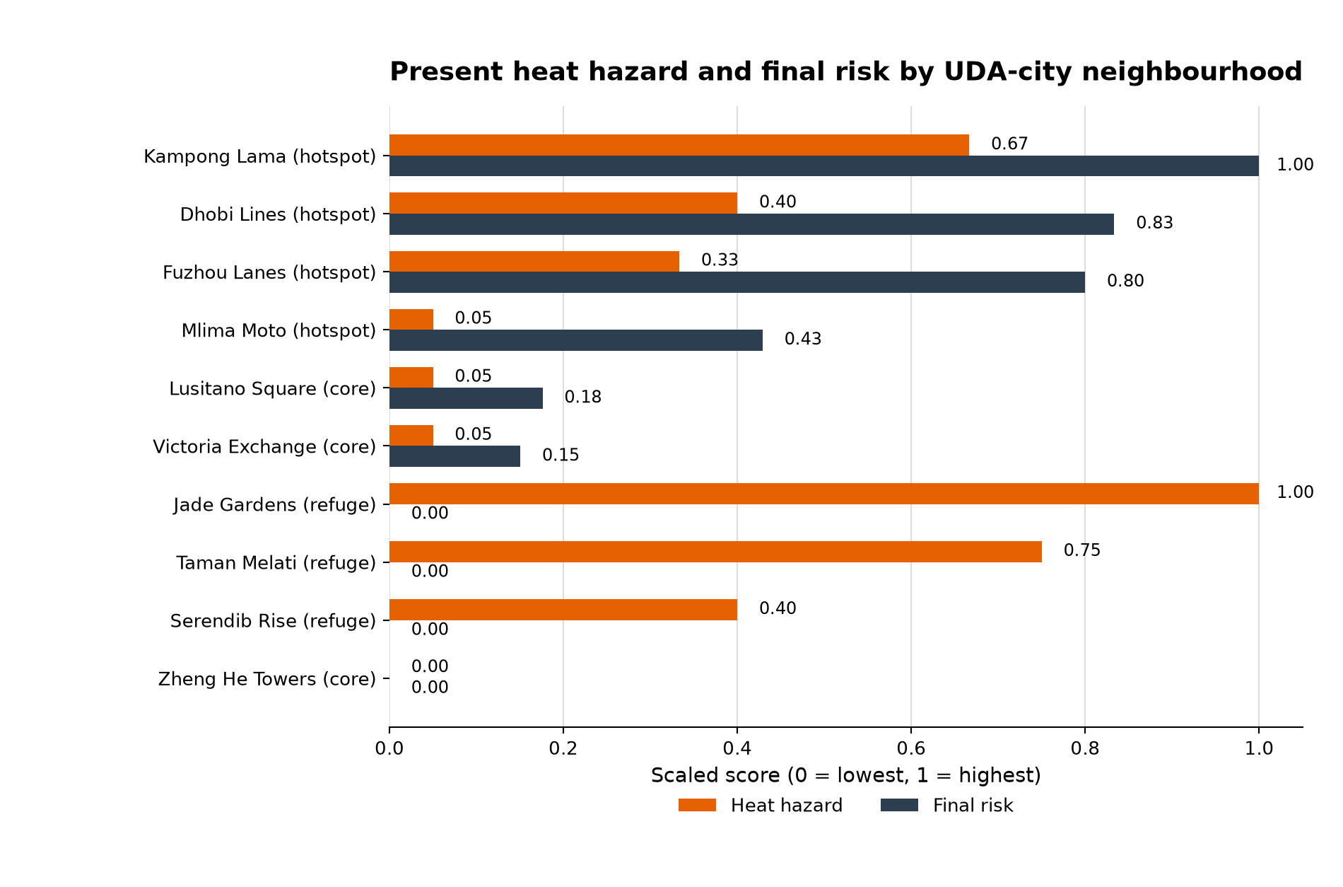Horizontal bar chart comparing scaled heat hazard and final risk for each UDA-city neighbourhood. Figure 1. Present-day heat hazard and final risk across UDA-city neighbourhoods. Both metrics are scaled from 0 to 1, where 1 is the highest value among the 10 neighbourhoods.

Key Results and Interpretation

Kampong Lama has the highest final heat-risk score because it combines substantial heat hazard with high exposure and high vulnerability.
Jade Gardens has the highest heat hazard with 62 dangerous-heat hours, but its final risk score is low because daytime population exposure is low.
Hotspot neighbourhoods dominate the top risk ranks, showing that social exposure and vulnerability strongly shape heat risk.
The ranking shows a heat hazard-risk paradox: the hottest neighbourhood is not necessarily the neighbourhood where people are most at risk.
These scores are relative rankings within UDA-city, so they compare the 10 neighbourhoods with each other rather than predicting absolute health outcomes.

Hazard-to-Risk Bridge

Where the bridge is scientifically strong

It separates physical heat hazard from social risk, which is important because the hottest place is not always the highest-risk place.
It combines hazard, exposure, and vulnerability, matching common climate-risk framing.
The method is transparent: each metric is scaled and the final risk formula is clear.
It is useful for comparing neighbourhood priorities inside the same synthetic city.

Where the bridge becomes weaker

It does not validate risk against observed health outcomes.
Vulnerability proxies may miss important factors such as health status, housing quality, access to cooling centres, or outdoor activity timing.
The geometric mean can hide details; a neighbourhood may rank high for different reasons than another.
Scaling within only 10 neighbourhoods means results are sensitive to the chosen study area.

SUEWS Citation

Jarvi, L., Grimmond, C.S.B. and Christen, A. (2011). The Surface Urban Energy and Water Balance Scheme (SUEWS): Evaluation in Los Angeles and Vancouver. Journal of Hydrology, 411(3-4), 219-237.

Ward, H.C., Kotthaus, S., Jarvi, L. and Grimmond, C.S.B. (2016). Surface Urban Energy and Water Balance Scheme (SUEWS): Development and evaluation at two UK sites. Urban Climate, 18, 1-32.